The Effect of Power and Confidence in Electronics Testing

Hypothesis Testing is the use of statistics for making rational decisions and I wanted to explore its use in test engineering. In doing so I found something very interesting that helps to support many of the ideas I’ve had. I should explain that the title of this article is a bit of a play on words as we will find out later.

Forming the Hypothesis¹

Let’s start at the beginning. We need to form a hypothesis about what it is we wish to know before designing a test. It is a supposition we might make about a population. We start by defining what is called the Null Hypothesis which is the thing that is normal and that which is most likely to occur, referred to as H0. It is assumed to be true unless there is strong evidence to the contrary. In the case of manufacturing we have:

H0 = observe samples from a population with no defect or faults.

Next we need to form an Alternative Hypothesis which must be measurable and mutually exclusive from H0 so that if one can occur the other cannot.  This is referred to as Ha. These sample observations must come from some cause.

Ha = observe samples from a population with defect or fault.

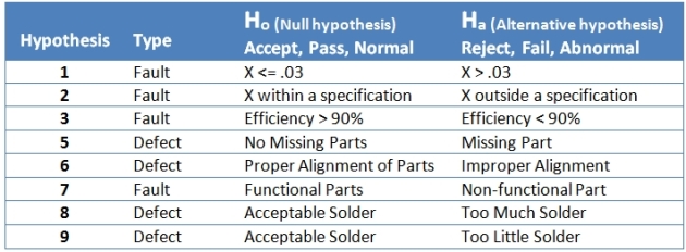
We have generalized a hypothesis in which we wish to prove that items produced by a manufacturing process are defect free (built correctly) and are without fault (working correctly). To elaborate, I’ve listed some hypotheses for H0 and Ha in Table 1 below.

Table 1 – Null and Alternative Hypotheses in Test Engineering

 

Hypothesis Testing²

Next we need to develop a test (or series of tests) to provide evidence for or against the null hypothesis.  Now, ‘evidence’ does not come from the null, which is the normal – a population (or item) without defect. ‘Evidence’ for our proof must come from the alternative hypothesis.

Following this line of reasoning we must understand that just because an item passes a test (for the null hypothesis) that it is conclusive evidence that there was no defect. This comes from the Power of the test to detect defects or faults (for the alternative hypothesis).  This is an important distinction to make because there are also sampling errors that can be made. The 4 outcomes of test which include errors are listed below.

Table 2 – 4 Conditional Outcomes of Test

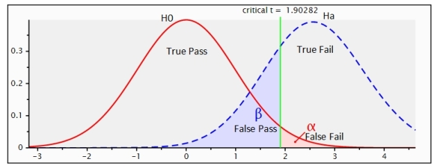
We can visualize the probability distributions for the null and alternative hypothesis by using a program called G*Power⁴.  In the figure below we see 2 normal distribution curves. The one on the left is the null hypothesis if the null is true. The curve on the right is for the alternative hypothesis if the alternative is true.

Figure 1 – Probability Distribution Curves for Null and Alternative Hypothesis

 

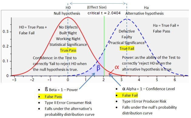
The areas shaded red and blue represent sampling errors under both hypotheses. The area shaded red is for the Type I Error (False Failures) for Producer Risk called Alpha α which is found under the null hypothesis. This is also called the level of significance. If the false failure rate (alpha) gets too high we begin to lose confidence that the test can provide evidence for the null hypothesis. Its complement is the Confidence Level where Alpha α = 1 – Confidence Level. If Alpha is 3% then Confidence would be 97%.⁵

 Confidence in the test (True Pass) comes from the level of significance found under H0.

The area shaded in blue lies under the alternative hypothesis. This is the Type II Error (False Passes) for Consumer Risk called Beta ß.  Beta is the complement of Power where ß = 1 – Power. If Power is 75% then Beta would be 25%.

 The ability of a test to correctly detect a defect (True Fail) is called Power found under Ha.

A third component represented in the figure above is the Effect Size. The further apart the distance between the 2 distributions, the higher the magnitude of the Effect, and the greater the evidence becomes for the alternative hypothesis when the alternative is true. Therefore, raising fault coverage (Power) has the direct effect of pushing the 2 distributions further away from each other.

Effect Size is the magnitude of the difference between H0 and Ha.

Now we have all 3 keywords used in the title for Confidence, Power and Effect. Figure 2 below puts everything together we have discussed up to this point.

Figure 2 – Hypothesis Test of Manufactured Items

 

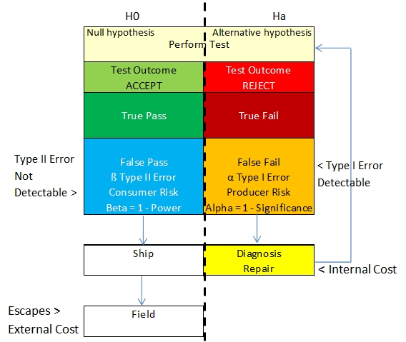
Referring to the Figure 3 below, let’s head out to the factory floor and see what happens. When we perform a test we will get 2 Results: ACCEPT or REJECT. Earlier we saw the 2 probability distributions for the null and alternative hypotheses. (Note: we are not talking about the defect rate.)

Figure 3 – Sampling Errors in the Test Process

 

We find that the Alpha Type I Error (False Fail, orange box) can be measured in the factory through the diagnostic/repair loop. You will find that Confidence in the test declines as the alpha error increases to a point where it becomes noticeable in your process.

But the Beta Type II Error (False Pass, blue box) cannot be measured on the factory floor. These errors get passed on to the next process or to the customer so its something you should know about. Since this sampling error cannot be detectable by the testing process we must do what is called a Power Analysis as it is Beta that controls the Type II Error. 

Power Analysis

As I have mentioned before in other articles, the closest thing we have is Fault Coverage. As for Power, I will attempt to translate what is done in clinical studies which can be used as a guideline in this situation.⁶

First, an a priori power analysis is usually done when designing a study. This is done to get the sample size needed in order to obtain a desired effect level. However, in manufacturing, the sample size is already defined by the central limit theorum.⁷

So, what we need is a way to computer Power. Perhaps we can compute Power through the use of fault simulation software. There are 2 pieces of information we must have. We must know the total number of defect opportunities that exist and we must know how many of those are defect opportunities are detectable by the test we are designing. It would be nice to have a simple, easy way to do this. All we would have to do is divide one by the other and get a decimal fraction from 0 to 1.0 that can be used as Power. However, this is quite difficult to do in practice. The reason is that every product and process is quite different while methods and standards are not well-established. But then this is a subject for another article.

Therefore, I have redefined the table for Power Analysis below based on its logical purpose for our situation.

Table 3 – Redefining Power Analysis in Test Engineering

 

Once the Power is known a Sensitivity Power Analysis can be undertaken where the Effect Size is calculated. As mentioned before, Effect Size is the magnitude of the difference between the 2 means measured in standard deviations. This can be useful in comparing different test cases to see how Power can be increased.⁸

For Criterion, we can measure alpha directly from the repair loop of our test process. Finally, here is an advantage that we have over research studies!

Post-hoc would be done on the testing process taken from real data to determine Beta. This data would come from downstream processes and field returns.

Alpha and Beta errors should have very little effect on each other in product testing. As an extreme example of this, we can say that it is possible to have 100% Power (for the alternative hypothesis) to find existing defects yet have 0% Confidence (in the null hypothesis) because faulty connections can result in an unacceptably high rate of false failures. We can also have 0% Power which would allow anything with a defect to pass yet have 100% Confidence and no false failures. In the first instance nothing gets through our test process while in the other everything gets through. I will leave it for you decide which of the two extremes seems worse and for whom.

Conclusion

I hope to have demonstrated the importance of Power to ‘provide evidence that the alternative hypothesis is true’.  We stated a hypothesis for testing manufactured items and through hypothesis testing, we looked at where sampling errors come from and described the need to do power analysis of fault coverage.

Yet Power Analysis has largely been overlooked due to the fact that it is difficult and time consuming to do with a scarcity of tools and methods that are available. Since methods are not well-established we find that testing generally takes place without much knowledge of Power or fault coverage. The reasons for this are as diverse and as varied as the companies and products they produce.

Power Analysis should be a matter of routine but many difficulties must still be overcome in both technology and mindset.

 

References

¹http://mathworld.wolfram.com/HypothesisTesting.html

http://onlinestatbook.com/2/logic_of_hypothesis_testing/significance.html

²http://statistics.about.com/od/Inferential-Statistics/a/Type-I-And-Type-II-Errors.htm

³Why do we say ‘fail to reject’? http://statistics.about.com/od/Inferential-Statistics/a/Why-Say-Fail-To-Reject.htm

⁴ G*Power statistical software http://www.gpower.hhu.de/

⁵Confidence levels are usually something that is selected by the researcher after setting a limit for alpha, usually 5%. However, in manufacturing we can measure alpha from the test process in real time. The detected defect rate gives us what is called the p-value. From the p-value we get a Z score as the area under the curve. This is the critical value shown in Figures 1 and 2. For example, say we select an alpha of .05 which is a Confidence Level of 95%.  This means we have decided that we will only tolerate false failures in our process of 5%. If the fallout rate from the test becomes greater than 5% we would be saying that we can no longer trust the test result when the outcome says to ACCEPT. We would be saying that for the test results to have statistical significance, the fallout rate from the test would have to be less than 5% in order to trust the test result when it says to ACCEPT. But this Confidence Level is subjective and will be relative to what you are comfortable with in your process as a higher alpha will result in greater internal costs. https://en.wikipedia.org/wiki/Statistical_significance

⁶ https://rgs.usu.edu/irb/files/uploads/A_Researchers_Guide_to_Power_Analysis_USU.pdf

⁷ https://en.wikipedia.org/wiki/Central_limit_theorem

⁸ Effect Size

https://researchrundowns.wordpress.com/quantitative-methods/effect-size/

http://staff.bath.ac.uk/pssiw/stats2/page2/page14/page14.html